Very Useful Microsoft Excel Tips and Short Cuts

Friends,

Now a days Excel is becoming a very useful part for Computers Users. In Excel there are so many functions with the help of those one can do his job very easily and comfortably which is even impossible if someone try to do it manually. While working in Excel. we need some shortcuts to do work fast. Here are some Excel Tips which could be very useful for doing job in Excel. Like as someone type some matter in Column mode but the Boss says to convert the Columns in Rows, then you don’t have to panic to type the matter again in Rows mode. Just use the following trick and convert it in just seconds.

• Convert Rows to Columns: You can convert rows to columns (and columns to rows) by highlighting the cells you want to switch around,clicking on Edit, Copy, selecting a new cell and then going to Edit, Paste Special… Finally, place a tick in the Transpose box on the dialog box and click on OK.
• Calculate time between dates: Enter in a cell the formula =A2-A1, where A1 is the earlier date, and A2 the later one. Don’t forget to convert the target cell to number format – do this by highlighting the cell, clicking on Format, Cells…, picking on the Number tab and selecting Number from the Category: list.
• Enter URLs as text, not hyperlinks: To prevent Excel from converting written Internet addresses into hyperlinks, add an apostrophe to the beginning of the address, for example ‘http://www.rajeshbaranwal.com.’
• Calculate Running Totals: Enter the numbers to be added in column A, say A1 to A5, then enter =SUM($A$1:A1) into column B. Highlight the cells beside the ones with numbers in (in our example, B1 to B5) and go to Edit, Fill, Down. This places the running total of the figures in A1 to A5 in the adjacent column.
• Remove Hyper links: From your work If Excel has already converted your written URL into a hyperlink, you can cancel it by right-clicking on the offending address and selecting Hyperlink, Remove Hyperlink from the menu that pops up.
• Fit wide tables to the page width: To make your tables fit neatly on the page, click on File, Page Setup…, select the Page tab, click on the Fit to:radio button and pick 1 page wide. Click on the tall box and press [Delete], leaving the box empty.
• Hide your data from prying eyes: If you want to hide from view any sensitive data, highlight the relevant cell and click on Format, Cells… Click on the Numbers tab, select Custom from the Category: list, double-click on the Type: input box and enter ;;;. Undo the operation to make your data visible again.
• Use template worksheets: Templates can save you considerable time when you’re setting up a new worksheet. Click on File, New…, select the Spreadsheet Solutions tab and choose a template from the list.
• Access help for Lotus users: If you have converted some worksheets from Lotus 1-2-3 and find Excel confusing, you can access help specific to your situation by clicking on Help, Lotus 1-2-3 Help…
• Use the formula browser: Select a cell and click on the Paste Function button on the main toolbar. Pick the function you require from the list box and click on OK. Now highlight the cells on which you want the target to perform the function and click on OK.
• Customise your AutoFills: If you use the same list over and over in different worksheets, you might want to add it to your AutoFill list – this will save you heaps of time in future. Highlight your list, click on Tools, Options… and select the Custom Lists tab. Click on Import, then OK.
• Use the Auto Calculator: If you need to calculate a sum based on a row or a column of figures and you can’t be bothered typing in a function, just select your figures and glance down at the status bar – you’ll find the sum of the selected cells there.
• A quick way to enter the time: To enter the current date or time click on a cell and type =today() or =now(). Excel updates the result every time you open the sheet, so it’s always current.
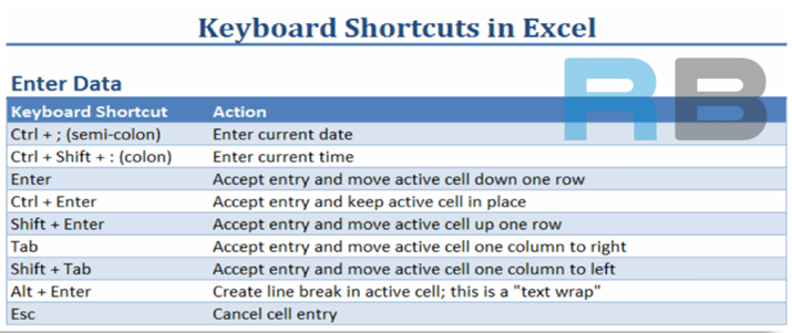
• Enter a fixed time into Excel: If you want Excel to enter the current date or time and fix it at that point – for example, to show the last date the sheet was modified – click on a cell and press [Ctrl] + [;] for the date and [Ctrl] + [:] for the time.
• Find the currently active cell: If you have been scrolling around your spreadsheet and you lose your place, you can jump back to the currently active cell by pressing the [Ctrl] + [Backspace] keys.
• See the big picture: If you’re working on a large sheet you might want to switch to Full Screen mode: simply click on View, Full Screen. Click on it again to return to a normal window.
• Fit text automatically: Make your work look neater by selecting the relevant column, and clicking on Format, Column, AutoFit Selection.
• Fast copy, no clipboard: Pressing [Ctrl] + [‘] is a speedy way to duplicate the formula or figure in the cell above the one you’re in.
• Fast and easy multiple entry: If you need to enter a formula in several cells at once, simply select all the target cells, type your formula as normal and press [Ctrl] + [Enter].
• Pick cells for Auto Calculator: You can select unconnected cells by holding down [Ctrl] while you click on the individual cells.
• Hide comments to reduce clutter: You can hide notes and other comments by using the Insert Comment function.Highlight a cell, click on Insert, Comment and type your text. Click away from the input box when you’ve finished. The comment will appear whenever you pass your mouse over the relevant cell.
• Re-colouring the grid lines: You can change the colour of the grid by clicking on Tools, Options…, selecting the View tab, clicking on the Color: list box and choosing a new colour from the palette. Choosing white effectively removes the grid completely.
• Angle your entries: To make Excel display the text in cells at an angle of 45 degrees, right-click on the toolbar, select Chart, and pick either of the ab icons on the new toolbar.
• To any degree you like: If you want custom angles right-click on the cell and select Format Cells… From the pop-up menu, click on the Alignment tab, and then drag the Text pointer in the Orientation window.
• Zoom in to your selection: You can have Excel display just the area you’re working in by highlighting the relevant cells, clicking on the arrow on the Zoom box on the toolbar and selecting Selection from the list.
• Another default entry direction: When editing cells the cursor moves down when you press [Return]. To change the direction click on Tools, Options… and select Edit. Click on the Move selection after Enter list box and choose another direction from the list.
• Launch Excel, open your file: Launch Excel, open the file you use most often, and click on File, Save As… In the Save As dialog, navigate to the Xlstart folder in your Office folder and click Save. Now the file will open automatically when you launch Excel.
• Set decimal points: Click on Tools, Options… and select the Edit tab. Place a tick in the Fixed decimal tick box and use the arrows in the Places: input box to set the number of decimal places.
• Calculate the median value: To calculate the median value of a number of figures, say A1 to A10, enter =median(A1:A10) into the target cell.
• #NAME! and #NUM! errors: Excel returns a #NAME! or #NUM! error whenever a formula refers to nonexistent names or numbers. To sort it out, re-enter the formula correctly.
• Quick sort your columns: The quickest way to sort a column into a hierarchy is to select it and click on  the Sort Ascending or Sort Descending buttons (the ones with the AZ arrows).
• Quickly change cell dimensions: The quickest way to change a column’s width or a row’s height is to place your mouse pointer close to the join between two columns or rows, then click and hold down the mouse button, and drag the column or row to the desired size .
• Erasing entries while typing: If you mistype your formula, press [Esc] to erase the cell’s content.
• Enter number sequences: Enter the first number in a cell, press the [Ctrl] key, and then click, hold and drag the cell’s handle until you have reached the desired number of cells.Release the mouse button first, and then the [Ctrl] key.
• See formulas at a glance: You can view all of your formulas at once by clicking on Tools, Options…, selecting the View tab, and placing a tick in the Formulas tick box.
• Highlight cells of a kind: You can select all the cells of a certain type by using the Special functions. Click on Edit, Go To…, click on the Special… button, choose the cell type from the dialog box and click on OK.
• Switch off the zeroes: You can prevent zeroes from cluttering your sheets by clicking on Tools, Options…, selecting the View tab, and unticking the Zero values tick box.
• Protect your work: Open the sheet you wish to protect and click on File, Save As… Click on the General Options… item in the Tools menu (in the top right corner of the Save As dialog) and enter a password in the Password to open: input box. Finally, click on the Save button. You might want to make a note of the password before continuing.
• Customize your dates: You can customize the format of a date in a cell using the Custom cell formatter. To do this, enter a date in a cell, click on Format, Cells…, click on Custom in the Category: pane, click on the Type: input box and press [M] repeatedly until the desired format is displayed in the Sample area above.
• Quick column copy: You can fill out the cells in a column by double-clicking on a cell’s handle.Excel will place copies of the clicked cell in each cell below, stopping when it reaches a cell with blanks either side.(Confused? Try this: enter a figure in cell A1, then enter figures in cells B1 to B5, then double-click on A1’s handle.)
• Merge cell contents: To merge the contents of cells A1 and B1, click on cell C1 and enter =A1&B1.The result is not a sum but a text string, so merging 10 and 7 will return 107, rather than 17.
• Use dynamic formatting: You can set Excel to alert you to critical figures in cells by setting it up so the colour or size of text in a given cell changes whenever a certain condition is reached. Select a cell (say, the cell containing the total of your bank balance) and click on Format, Conditional Formatting… Choose the conditions in the pop-up dialog (say ‘Cell value is less than 0’) and click on the Format… button. Now choose a new colour in the Color: list box and click on OK. Click on OK again to finish. From now on Excel will display your chosen figure in the new colour whenever the figure falls below zero.
• Border connected cells: You can place a border around a group of related cells – all the totals, for example – by selecting them and clicking on Format, Cells…, then selecting the Border tab and clicking on the Outline button.
• Shrink entries to fit their cells: You can force Excel to display the full text of a cell by using the Shrink to fit option. Click on Format, Cells…, click on the Alignment tab and place a tick in the Shrink to fit tick box. Obviously, the more text you have, the smaller it’ll be, so this isn’t practical for small cells with lots of content.
• Create hyperlinks to support files: To place links in cells that enable you to load other documents with one click, enter a name for the link in a cell and press [Ctrl] + [K]. Click on the File… button. Navigate to the file you wish to link to. Double-click on it and click OK. From now on, whenever you click in that cell, Excel will jump to the file.

I think these short cut functions of Excel will help you.  Kindly note that these commands are may not be workable in all excel version but most of versions have this features.Further there is only on method/ procedure to solve one query is given though there are more than one methods in excel to do same thing.